A new page for our Market Dashboard
If you follow us for a while you might have encountered one of our posts related to the FED’s target interest rate hikes, where we show the expected interest rate hikes for each of this year’s FED meetings.
With its great underlying information, this was a natural fit as the second feature for the app.
During the process, we make use of the following packages:
shinyfor the UIDBIfor writing to and querying our databasepolitefor politely asking websites to scrapervestfor webscrapingdplyr,stringrandlubridateas utilitiesplotlyfor interactive visualization
Data retrieval
If you ever have heard about ETL-processes, our data retrieval is a very basic idea of it. ETL stands for “Extract, Transform, Load” and simply means get data from somewhere, fiddle around with it for your needs and then put it into some storage for later use. To understand this a bit better I will go through the complete process.
E - Extract
For this project, we need to extract data from two different locations. First, the FED’s meeting dates we get from the FED’s website (unfortunately, there is no information about 2023 meetings).
This is how the website looks: 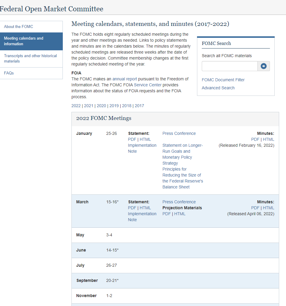
And this is the code we use to extract the data
# FED Meetings
url <- "https://www.federalreserve.gov/monetarypolicy/fomccalendars.htm"

#Check robot.txt, get approval and establish a session
fed_session <- polite::bow(url, force = FALSE,verbose = TRUE, delay = 5)

fed_df <- polite::scrape(fed_session) %>%
  rvest::html_node(".panel.panel-default") %>%
  rvest::html_nodes(".row.fomc-meeting") %>%
  rvest::html_text() %>%
  stringr::str_remove_all("\\r|\\n") %>%
  stringr::str_remove_all("\\*") %>%
  stringr::str_squish() %>%
  dplyr::as_tibble() %>%
  tidyr::separate(col = value, sep = " ", into = c("month", "date")) %>%
  dplyr::mutate(month_no = match(month, month.name),
                date = as.integer(stringr::str_extract(date, "(?<=-).*"))) %>%
  dplyr::mutate(meeting_date = paste0(
    lubridate::year(lubridate::today()),"-",month_no,"-",date)
    ) %>%
  dplyr::filter(meeting_date > lubridate::today())

fed_df
## # A tibble: 6 x 4
## month date month_no meeting_date
## <chr> <int> <int> <chr>
## 1 May 4 5 2022-5-4
## 2 June 15 6 2022-6-15
## 3 July 27 7 2022-7-27
## 4 September 21 9 2022-9-21
## 5 November 2 11 2022-11-2
## 6 December 14 12 2022-12-14We are using the awesome polite package for responsible scraping. In short, it scans the robots.txt of a website for scraping rules and asks for permission to scrape, but check it out yourself for more details. With the help of rvest and the tidyverse we get a nice output.
After we got the meeting dates, we can now scrape the future data which we need for calculating the implied rate changes. The future data is available on ino.com. Thankfully, the values are wrapped into a HTML table, so extracting is not difficult. This is the site:
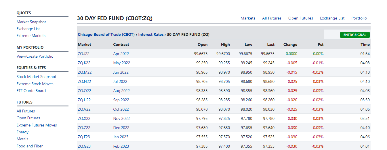
Again, we use polite to introduce us to ino.com first and then just scrape the table from the website.
# Scrape INO for future prices --------------------------------------------

url <- "https://quotes.ino.com/exchanges/contracts.html?r=CBOT_ZQ"

#Check robot.txt, get approval and establish a session
session <- polite::bow(url, force = FALSE,verbose = TRUE, delay = 5)

#Get price and time information
price <- polite::scrape(session) %>%
  rvest::html_table(header = FALSE) %>%
  .[[1]] %>%
  janitor::row_to_names(row_number = 3,
                        remove_row = T,
                        remove_rows_above = T)

price
## # A tibble: 145 x 9
## Market Contract Open High Low Last Change Pct Time
## <chr> <chr> <chr> <chr> <chr> <chr> <chr> <chr> <chr>
## 1 ZQ.J22 Apr 2022 99.6700 99.6725 99.6700 99.6700 -0.0025 -0.00% 17:28
## 2 ZQ.K22 May 2022 99.230 99.230 99.225 99.230 0.000 0.00% 07:03
## 3 ZQ.M22 Jun 2022 98.885 98.885 98.875 98.885 0.000 0.00% 07:02
## 4 ZQ.N22 Jul 2022 98.555 98.565 98.545 98.565 +0.010 +0.01% 07:05
## 5 ZQ.Q22 Aug 2022 98.155 98.160 98.140 98.160 +0.010 +0.01% 07:04
## 6 ZQ.U22 Sep 2022 98.040 98.040 98.020 98.040 +0.005 +0.01% 07:04
## 7 ZQ.V22 Oct 2022 97.760 97.780 97.750 97.770 +0.005 +0.01% 07:05
## 8 ZQ.X22 Nov 2022 97.520 97.540 97.500 97.530 +0.005 +0.01% 07:07
## 9 ZQ.Z22 Dec 2022 97.390 97.410 97.365 97.395 +0.005 +0.01% 07:03
## 10 ZQ.F23 Jan 2023 97.290 97.325 97.275 97.310 +0.010 +0.01% 07:03
## # ... with 135 more rowsThis marks the end of our Extract phase.
T - Transform
The data transformation is now done with our utility tools dplyr, tidyr, stringr, lubridate and janitor.
As there are future prices and spreads in the same table, we first separate the Contract column into a from and a to column, wherever contract_to is empty, we set the fut_type to “price”, otherwise “spread”. Adding a retrieval_date helps us identifying unique values. Because the HTML table stores everything as a character we use dplyr::across() to convert the numeric columns to type double.
As the name suggests, janitor::clean_names tidies the column names to lowercase and if there are spaces, concatenates the names with underscores. Finally, we delete one line containing values we don’t need.
# Prepare data for DB upload ----------------------------------------------

cleaned_table <- suppressWarnings(price %>%
  dplyr::as_tibble() %>%
  tidyr::separate(Contract,into = c("contract_from","contract_to"), sep = "\\/") %>%
  dplyr::mutate(retrieval_date = lubridate::now(),
                fut_type = ifelse(is.na(contract_to),"price","spread"),
                contract_to = stringr::str_remove(contract_to, " Spread"),
                Pct = stringr::str_remove(Pct, "%"),
                from_month = lubridate::month(lubridate::my(contract_from)),
                from_year = lubridate::year(lubridate::my(contract_from)),
                dplyr::across(.cols = c("Open","High","Low","Last","Change","Pct"),
                              .fns = as.numeric),
                Pct = Pct/100,
                source = "quotes.ino.com") %>%
  janitor::clean_names() %>%
  dplyr::rename(ticker = market) %>%
  dplyr::filter(!stringr::str_detect(ticker,"All quotes"))
)

DT::datatable(cleaned_table,
               rownames = FALSE,
               options = list(pageLength = 5,
                              scrollX = T))
L - Load
The final step is just to load the transformed data into our own database, which is really easy thanks to the DBI package. We use a small check before writing in order to avoid getting duplicates.
# Database upload --------------------------------------------------------

mydb <- connect_to_DB() #Own wrapper for DBI::dbConnect with safely stored credentials

# Check the current months ticker
check_ticker_date <- relevant_ticker(month = lubridate::month(lubridate::today()),
                                     year = lubridate::year(lubridate::today()))

# Get max retrieval date for this ticker
max_db_date <- DBI::dbGetQuery(mydb, paste0("SELECT MAX(retrieval_date) AS max_db_date
                                             FROM eco_fed_funds_future_prices
                                             WHERE ticker = '",check_ticker_date,"'")) %>%
  dplyr::mutate(max_db_date = lubridate::as_date(max_db_date))

# write to DB if not done yet
if(max_db_date$max_db_date < lubridate::today()){
      DBI::dbWriteTable(mydb,
                        name = "eco_fed_funds_future_prices",
                        value = cleaned_table,
                        append = TRUE,
                        row.names = FALSE)
}
Now the ETL process is finished. The database looks like this:
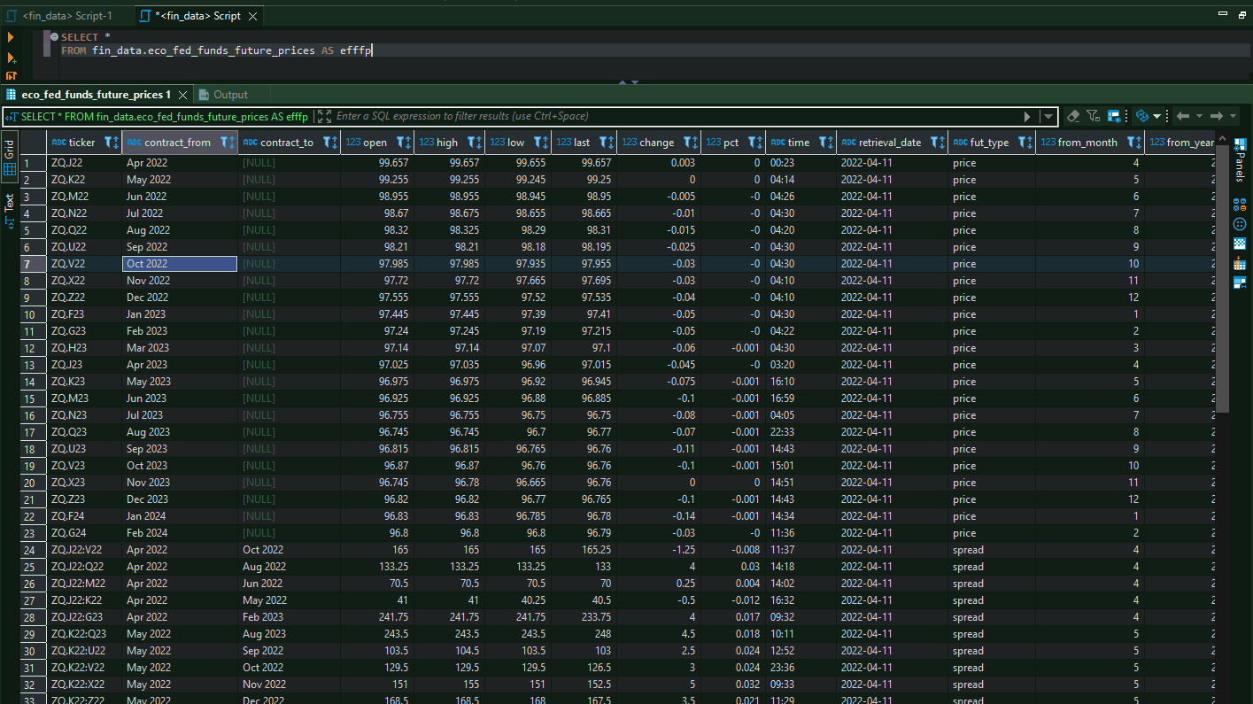
And we can start calculating our hike probabilities
The Implied Hikes
For the probabilities of a rate hike we need to take some basic assumptions. The website of the CME explains the whole process very good.
For an overview, this are the three main assumptions:
Probability of a rate hike is calculated by adding the probabilities of all target rate levels above the current target rate.
Probabilities of possible Fed Funds target rates are based on Fed Fund futures contract prices assuming that the rate hike is 0.25% (25 basis points) and that the Fed Funds Effective Rate (FFER) will react by a like amount.
FOMC meetings probabilities are determined from the corresponding CME Group Fed Fund futures contracts.
And the formula for the probability is
P(Hike) = [ FFER(end of month) – FFER(start of month ) ] / 25 basis points
For a deeper dive into the calculations we refer to the CME’s Methodology page linked above.
Our implementation in R uses a function which calculates the key figures
- Implied Rate
- Probability of a rate change
- Probability of no rate change
for a given FED meeting.
get_hike_prob <- function(meeting=NULL, previous_month_price=NULL){


  # Link to CME Methodology:
  # https://www.cmegroup.com/education/demos-and-tutorials/fed-funds-futures-probability-tree-calculator.html

  cat(cli::col_magenta("Calculate Probabilities for ", meeting, "\n"))

  if(is.null(meeting)){
    stop("No Meeting Date set")
  }

  month <- lubridate::month(meeting)
  year <- lubridate::year(meeting)


  # Find the correct Fed Fund Future Ticker
  actual_ticker <- relevant_ticker(month, year)

  if(month == 1){
    previous_ticker <- relevant_ticker(12, year-1)
  } else {
    previous_ticker <- relevant_ticker((month-1), year)
  }
  if(month < 12){
    nxt_ticker <- relevant_ticker(month+1, year)
  } else{
    nxt_ticker <- relevant_ticker(1, year+1)
  }


  # Get the prices
  act_month <- get_future_prices(actual_ticker)

  pre_month <- get_future_prices(previous_ticker)

  nxt_month <- get_future_prices(nxt_ticker)

  N <- lubridate::days_in_month(meeting)[[1]] #Days in Meeting Month
  M <- lubridate::day(meeting)-1 #Days in month till meeting


  if((month+1) %in% fed_df$month_no){
    # Type 2 Meeting - References to CME methodology
    FFER_start <- 100 - pre_month
    implied_rate <- 100 - act_month

    FFER_end <- (N/(N-M)) * (implied_rate - (M/N) * FFER_start)

  } else {
    # Type 1 Meeting
    implied_rate <- 100 - act_month
    FFER_end <- 100 - nxt_month
    FFER_start <-  (N/M) * (implied_rate - (((N-M)/N) * FFER_end))

  }

  #Probability of Rate change in Meeting
  p_change <- (FFER_end - FFER_start) / 0.25


  # Check if Hike (p>0), or cut (p<0)
  if(sign(p_change)==1|sign(p_change)==0){
    p_unchange <- 1 - p_change
    type = "hike"
  }else{
    p_unchange <- 1 + p_change
    type <- "cut"
  }

  probs <- tibble::tibble("retrieval_date" = lubridate::today(),
                          "meeting_date" = lubridate::as_date(meeting),
                          "p_change" = p_change,
                          "p_nochange" = p_unchange,
                          "impl.rate" = FFER_end,
                          "type" = type)
  return(probs)

}
With the magic of purrr we loop this function over every meeting date we got from the FED’s website and aggregate the total number of expected rate hikes as the cumulative sum of p_change as suggested in the general assumptions:
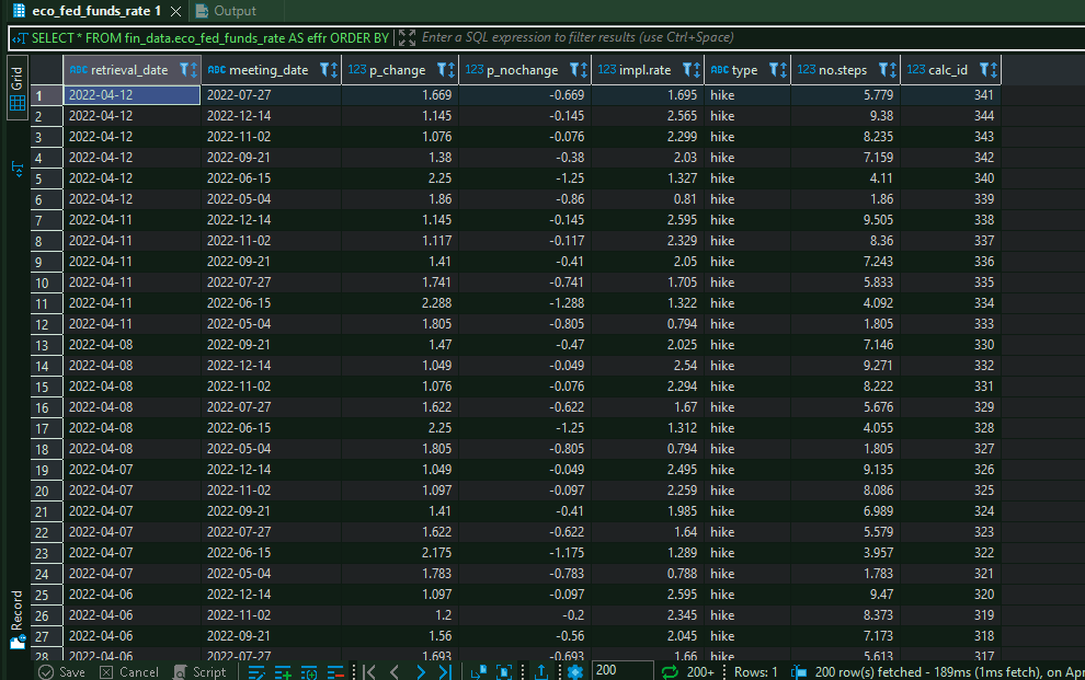
meeting_probs <- purrr::map_df(all_meetings, get_hike_prob) %>%
  dplyr::mutate(no.steps = cumsum(p_change))
The result gets written to another database table, from where we will retrieve it in our next and last step.
The app
After taking a long way, we finally have the needed data we want to display. Due to all the pre-processing, in our app we just need to load our FED figures from the database and can focus on building an interactive visualization of it.
Here, we use plotly for making an interactive graphic.
In our ui.R file, we first define the UI logic with two dateInput buttons for comparing two rate curves and then output the plotly we generate on the server side.
            shinydashboard::tabItem(tabName = "fed_funds",
                                    h2("Fed Funds Rates"),

                                    shiny::fluidRow(
                                      shiny::h3("Market Forward Curve Expectation"),

                                      shiny::column(width = 2,
                                      # Select 1st Date
                                      shiny::dateInput(inputId = "fed_date_1",
                                                       label = "Select Valuation Date for 1st Curve",
                                                       value = lubridate::as_date(
                                                         bizdays::offset(lubridate::today(),
                                                                         -1,
                                                                         'UnitedStates/NYSE')
                                                       ),
                                                       format = "dd.mm.yyyy",
                                                       daysofweekdisabled = c(0,6))
                                      ),

                                      shiny::column(width = 2,
                                      # Select 2nd Date
                                      shiny::dateInput(inputId = "fed_date_2",
                                                       label = "Select Valuation Date for 2nd Curve",
                                                       value = lubridate::as_date(
                                                         bizdays::offset(lubridate::today(),
                                                                         -2,
                                                                         'UnitedStates/NYSE')
                                                       ),
                                                       format = "dd.mm.yyyy",
                                                       daysofweekdisabled = c(0,6))
                                      )
                                      ),
                                    shiny::fluidRow(

                                      plotly::plotlyOutput("fed_rates") %>%
                                        shinycssloaders::withSpinner(),
                                      "Note: 1 hike = 25bps rate step"
                                    )
            )
In the server.R, we need a reactive value that listens to the dateInputs from the UI side. With this inputs it then calls the function get_fed_rates_fun which we define in our functions file.
server.R
  fed_rates <- shiny::reactiveVal(NULL)


  shiny::observe({

    fed_rates_plotly <- get_fed_rates_fun(input$fed_date_1,
                                         input$fed_date_2)

    fed_rates_plotly
    plotly::event_register(fed_rates_plotly, "plotly_click")

    fed_rates(fed_rates_plotly)

  })

  output$fed_rates <- plotly::renderPlotly({
    fed_rates()
  })
functions.R
get_fed_rates_fun <- function(date1 = NULL, date2 = NULL){

  mydb <- connect_to_DB()

  if(!is.null(date1)){
  fed_curve_date1 <- DBI::dbGetQuery(mydb,
                  stringr::str_c(
                    "SELECT *
                  FROM fin_data.eco_fed_funds_rate
                  WHERE date = '",date1,"'"))
  }

  if(!is.null(date2)){
  fed_curve_date2 <- DBI::dbGetQuery(mydb,
                                     stringr::str_c(
                                       "SELECT *
                  FROM fin_data.eco_fed_funds_rate
                  WHERE date = '",date2,"'"))
  }

  fed_plotly <- plotly::plot_ly(
    data = fed_curve_date1,
    name = date1,
    x = ~meeting_date,
    y = ~no.steps,
    text = ~p_change,
    type = "scatter",
    mode = "lines+markers",
    line = list(
      color = main_color),
    marker = list(
      color = main_color),
    hovertemplate = paste0("<extra><b>Curve Date: ",date1,"</b><br>Combined expected hikes: %{y:.2f}<br>Expected hikes in this meeting: %{text:.2f}</extra>")) %>%
    plotly::add_annotations(
      data = fed_curve_date1,
      x = ~meeting_date,
      y = ~no.steps + 0.5,
      text = ~ scales::percent(p_change, accuracy = 0.01),
      showarrow = FALSE,
      font = list(
        color = main_color
      )
    )

  if(!is.null(date2)) {

    fed_plotly <- fed_plotly %>%
      plotly::add_trace(
      data = fed_curve_date2,
      name = date2,
      x = ~meeting_date,
      y = ~no.steps,
      type = "scatter",
      mode = "lines+markers",
      line = list(
        color = palette_main[4]),
      marker = list(
        color = palette_main[4]),
      hovertemplate = paste0("<extra><b>Curve Date: ",date2,"</b><br>Combined expected hikes: %{y:.2f}<br>Expected hikes in this meeting: %{text:.2f}</extra>")) %>%
      plotly::add_annotations(
        data = fed_curve_date2,
        x = ~meeting_date,
        y = ~no.steps - 0.5,
        text = ~ scales::percent(p_change, accuracy = 0.01),
        showarrow = FALSE,
        font = list(
          color = palette_main[4]
        )
      )

  }

  plotly_output <- fed_plotly %>%
    plotly::layout(
      xaxis = list(
        title = "FED Meeting Date"
      ),
      yaxis = list(
        title = "No. of Implied Rate Hikes"
      ),
      hovermode = "x unified"
    )
  DBI::dbDisconnect(mydb)
  return(plotly_output)

}
This now results in our final plotly output when navigating to the new FED Funds Rate tab.
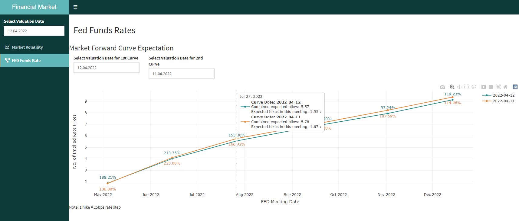
And thats the whole process behind this new addition to our Financial Market Dashboard.
What do you think about the FED Funds tool? We’d love to hear your feedback and are always happy to answer your questions.
Check out the About Page for our contact information or write us directly via mail.